GLPK Scheduling
This page contains notes on the use of Integer Linear Programming (ILP) to obtain a solution for a classic sequential job scheduling problem. This begins with a small discussion of ILP, followed by a description of the problem and an implementation of its formulation using the Haskell GLPK bindings. A solution to an example problem instance is provided at the end of the page. The content here is an introduction. A comprehensive treatment of ILP and scheduling is offered by [1].
Linear Programming
Linear Programming (LP) and its integer and mixed precision variants are classic mathematical optimization techniques. Together, they constitute an important part of the model-based family of approaches to optimization. Given known problem parameters A \in \mathbb{R}^{m \times n}, b\in \mathbb{R}^m and c \in \mathbb{R}^n, the LP setting is the following:
{\displaystyle { \begin{aligned}& {\text{minimize}}&&\mathbf {c}^{\top} \mathbf {x} \\ &{\text{subject to}}&&A\mathbf {x} \leq \mathbf {b} \\ &&&\mathbf {x} \geq \mathbf {0}. \end{aligned} } }
Where x is the design variable of the problem, i.e. the quantity we’re trying to determine, which is usually a vector. There are a few classical cases for x:
- When x\in \mathbb{R}^n is a real-valued vector, the problem setting is called Linear Programming(LP). LP is a tractable setting for which algorithms of polynomial complexity in m and n are known. This is true for both the optimization and constraint satisfactionThe “constraint satisfaction” version of the problem setting consists in finding an x such that the constraint A\mathbf{x} \leq \mathbf{b}, \mathbf{x} \leq \mathbf{0} is satisfied, if such an x exists.
versions of the problem.
When x \in \mathbb{Z}^n is an integer vector, the problem setting is called Integer Linear Programming (ILP) and no polynomial time algorithm in m or n is known. This is true for both the minimization and constraint satisfaction versions of the problem.
When x is a part integer- and part real-valued vector, the problem setting is called Mixed-Integer Programming (MIP) and the complexity situation is similar to that of ILP.
While don’t have a polynomial algorithm for the integer variants of this problemIf we did have one, we’d know that P=NP
, a number of things can be done in practice with ILP and MIPs:
Exact algorithms can be used with computational budgets. Such algorithms may terminate quickly despite their exponential worst case complexity. When such an algorithm indeed terminates, the solution it returns is guaranteed to be optimal for the problem instance.
Heuristics can also be used. They usually outperform exact algorithms for some problem instances. Because ILP is NP-Complete, their worst case run-time is still exponential though. Additionally, they don’t guarantee optimality if and when a result is returned.
A relaxation of problem instances to the LP setting turns out to be useful. The so-called “LP relaxation” of an integer-valued program is the corresponding real-valued (in x) version of the formulation. When the relaxed problem is satisfiable, its optimal value is guaranteed to be a lower bound on the optimal value of the original problem. Because LP is tractable, such a lower bound can be obtained easily in practice. When the relaxed problem formulation is unsatisfiable, we have a proof that the integer-constrained version of the problem is also unsatisfiable.
glpk-hs provides Haskell support for linear programming in the form of a shallowly embedded DSL for the CPLEX LP format and bindings to the GLPK solver. The code snippets in this page will use this package. The following section describes a classic scheduling problem we’ll look to transcribe under the ILP setting.
A classic scheduling problem
Consider the following: We’d like to schedule some sequential jobs on some heterogeneous resources. Jobs have precedence constraints, meaning that some jobs must finish before others can start. Each resource is only able to run a subset of the jobs, and a job run-time is function of the resource it is assigned to. This is a classic problem, for which some good method-based approachesThe HEFT[3] heuristic is designed specifically for this problem. Note that this heuristic considers a problem with communication times, which we are not considering here. Those can also be encoded in an ILP formulation, as is done in [2].
are known.
We’ll work with full a-priori information about our problem, meaning that the following parameters are all static and known in advance:
A set of jobs J, resources R and precedences P.
j \in J must precede job k \in J if there exists (j,k) \in P \subset J\times R. Suppose this constitutes a directed acyclic graph, meaning that there are no cyclical job dependencies.
Resource-job compatibility parameters v_{jr} \in \{0,1\} of job j\in J and resource r\in R. We have v_{jr}=1 when j is compatible with r, and v_{jr}=0 otherwise.
Processing time p_{jr} \in \mathbb{N} for job j\in J on resource r \in R.
Suppose we want to schedule jobs as fast as possible, for the following definition of fast: We want to minimize the makespan of the schedule as our objective, defined as the latest completion time of all jobs in the schedule. Now that we’ve defined our problem and assigned some notation for its parameters, let’s move on to the ILP formulation.
ILP Formulation
We want to write the following function that takes the problem parameters as input and returns a value of type LP, which represents an instance of a problem. The type of the function we’ll be writing in the rest of this page is the following:
Extensions, imports and helpers
{-# LANGUAGE GeneralizedNewtypeDeriving #-}
{-# LANGUAGE OverloadedLists #-}
{-# LANGUAGE ParallelListComp #-}
{-# LANGUAGE ScopedTypeVariables #-}
{-# OPTIONS_GHC -fno-warn-orphans #-}

module Sched where

import Algebra.Classes
import Control.Lens hiding (op)
import Control.Monad.Writer
import Data.LinearProgram
import qualified Data.Map as M
import Protolude hiding (Num (..))
import qualified Protolude (Num (..))
import Prelude (String)

type Time = Int
-- ^ Builds a set of precedence edges from an adjacency list map.
expandMap :: Map a [a] -> [(a, a)]
expandMap = mconcat . fmap (\(x, xs) -> (fmap (x,) xs)) . M.toList-- ^ The cartesian product of two lists.
cartesian :: [a] -> [b] -> [(a,b)]
cartesian a b = (,) <$> a <*> b-- ^ A linear combination with one term of weight 1.
single :: (Ord v, Additive r, Protolude.Num r) => v -> LinFunc v r
single x = linCombination [(1, x)]formulation
:: forall job resource
. (Eq job, Show job, Show resource)
=> Set job -- ^ Jobs we need to schedule.
-> Set resource -- ^ Resources we can schedule on.
-> Map job [job] -- ^ Job precedence constraints.
-> (job -> resource -> Bool) -- ^ Whether a job can run on a given resource.
-> (job -> resource -> Time) -- ^ Time a job takes to run on on a resource.
-> Time -- ^ Makespan upper bound.
-> LP String Int -- ^ The LP program.Let’s start with the design variables of our problem.
Design variables
We’ll use two sets of design variables. One for allocation (x_{jr}, written as allocated), and one for start times (s_j \in \mathbb{N}, written as startTime)For the sake of simplicity we’ll assume the Show instances for the job and resource types are so that show is surjective for each instance. This way, we don’t have to think about how to supply unique variable names. Expand the “Supply helpers” code block for details.
.
Supply helpers
lpShow :: Show a => a -> String
lpShow x = go <$> show x
  where
    go ' ' = '_'
    go y = y
sub2 :: (Show a, Show b) => String -> (a, b) -> String
sub2 x (y, z) = x <> "_" <> lpShow y <> "_" <> lpShow z
sub :: (Show a) => String -> a -> String
sub x z = x <> "_" <> lpShow zallocated :: (Show job, Show resource) => (job, resource) -> String
allocated = sub2 "x"
startTime :: Show job => job -> String
startTime = sub "s"We’ll later need two more design variables to express constraints and objectives, so let’s define those already.
tau_ :: (Show a, Show b) => (a, b) -> String
tau_ = sub2 "Theta"
cMax :: String
cMax = "C_max"We’ll bind variables as such:
formulation
  (toList -> jobs :: [job])
  (toList -> resources :: [resource])
  (expandMap -> precedences :: [(job, job)])
  (uncurry -> compatible)
  (uncurry -> processingTime)
  makeSpanBound = execLPM $ do
Where expandMap :: Map a [a] -> [(a, a)] builds a set of precedence edges from an adjacency list map.
allocation : x_{jr} = 1 \text{ if } j \in J \text{ assigned to } r \in R. This is expressed using the setVarKind primitive that sets variable boundsIn this snippet and the below, we denote the cartesian product by cartesian :: [a] -> [b] -> [(a,b)].
:
    sequence_
      [ setVarKind (allocated jr) BinVar
      | jr <- cartesian jobs resources
      , compatible jr
      ]
Note that we don’t declare this binary variable for cases where v_{jr} = 0. We’ll make those variables redundant by construction later.
start times : s_j \in \mathbb{N}:
    for_ jobs $ \ (startTime -> s_j) -> do
      setVarKind s_j IntVar
      s_j `varGeq` 0
where startTime :: Show job => job -> String is our variable naming convention for s_j, and other primitives are self-explanatory.
Objective
The makespan of the schedule is the maximum completion time of all jobs. We’ll define this using a constraint, but for now let us just declare a corresponding variable and indicate it will serve as the quantity to be minimized:
    setVarKind cMax ContVar
    setObjective $ single cMax
    setDirection Min
Where single is a helper that lifts a single design variable to a constraint, setDirection and setObjective are primitives used to set-up the problem, and cMax :: String is our variable name for the objective.
Constraints
The first constraint is an objective in disguise.
makespan definition: The makespan is the maximum job completion time.
For any job j\in J and resource r \in R such that v_{jr}>0, one has the following constraint:Expressing the maximum function via a constraint is a a standard trick for coercing the LP problem setting into admitting this kind of objective function.
\quad C_\text{max} \geq s_j + p_{jr} x_{jr}
    sequence_
      [ linCombination
          [ (-1, cMax)
          , (1, startTime j)
          , (processingTime jr, allocated jr)
          ]
        `leqTo` 0
      | jr@(j, _) <- cartesian jobs resources
      , compatible jr
      ]
We now express constraints that ensure the solution respects the geometry of the scheduling problem.
unique assignment: Each job is assigned to exactly one resource.
For any job j\in J, one has \sum_{r \in R} x_{jr} = 1. This is in reality two inequalities in hiding. glph-hs exposes the equalTo primitive for this transformation:
    for_ jobs $ \j ->
      linCombination [(1, allocated (j, r)) | r <- resources] `equalTo` 1
resource/job compatibility: A job can only run on a compatible resource.
For any job j \in J and resource r \in R such that v_{jr}=0, one has x_{jr}=0.
    sequence_
      [ single (allocated jr) `equalTo` 0
      | jr <- cartesian jobs resources
      , not (compatible jr)
]precedences: A job can not start before its predecessors have terminated.
For any r\in R and (j,k) \in J such that v_{jr}=1 and there exists a precedence relation (j,k) \in P, one has s_k \geq s_j + p_{jr} x_{jr}.
    sequence_
      [ linCombination
         [ (1, startTime k)
         , (-1, startTime j)
         , (-(processingTime jr), allocated jr)
         ]
        `geqTo` 0
      | (j, k) <- precedences
      , r <- resources
      , compatible (j, r)
      , let jr = (j, r)
]over-commitment: Resources should not be over-committed.
This one is trickier to express. For any two jobs (j,k)\in J, define the overlap O_{jk} of job j on job k to be O_{jk} = s_k - \sum_{r\in R} p_{jr} x_{jr} - s_j, and consider the following graph for two jobs allocated to the same resource, where jobs are overlapping.
\quad
j   |------------------------------------|
k   .        |--------------------------------------------|
    .        .                           .                .
    .        .          O_jk             .                .
    .        <--(negative direction)------                .
    .                                                     .
    <-----(negative direction)-----------------------------
                   O_kj
For any (j,k)\in J, j and k overlap if and only if O_{kj} < 0 and O_{jk} < 0. We need to express a NAND constraint on those two inequalities. It is not immediately obvious how to do so, but fortunately we have another trick in our bag.
We introduce \tau_{jk} \in \{0,1\}, indicator variable for O_{jk} + 1 \leq 0 and for any (j,k) \in J specify that O_{jk} + 1 \leq u(1- \tau_{jk}) and O_{jk} \geq -u \tau_{jk}, where u \in \mathbb{N} is any upper bound on the left-side quantities. This allows to express semantics for \tau_{jk}. Re-formulated, this corresponds to the following set of constraints and variable definitions. For any (j,k) \in J such that j \neq k, one has:
s_k - \sum_{r\in R} p_{jr} x_{jr} - s_j + 1 \leq u(1- \tau_{jk}),
s_k - \sum_{r\in R} p_{jr} x_{jr} - s_j \geq - u \tau_{jk},
\tau_{jk} \in \{0,1\}.
where u is an upper bound on the overlap - which is maximally equal to the makespan of the solution. We’ll use the upper-bound on the makespan obtained from the signature of formulation.
    sequence_
      [ do
          setVarKind (tau_ (j, k)) BinVar
          tauConstraint `geqTo` 0
          tauConstraint `leqTo` (makeSpanBound - 1)
      | (j, k) <- cartesian jobs jobs
      , j /= k
      , (j, k) `notElem` fullPrecs
      ,  let tauConstraint =
                single (startTime k)
              - single (startTime j)
              + linCombination [(makeSpanBound, tau_ (j, k))]
              - linCombination
                  [ (processingTime (j, r), allocated (j, r))
                  | r <- resources, compatible (j, r)
                  ]
      ]
Note that some of those constraints were already enforced by job precedence constraints. An easy way to reduce the number of constraints is to omit any such constraint between jobs (j,r)\in J where j and r have an indirect precedence relation in the DAG. Assume that we have computed such a set of indirect precedence relations called fullPrecs, which we used to guard our list comprehension. Remains to express the NAND constraint on O_{kj} < 0 and O_{jk} < 0:
For any r \in R, (j,k) \in J s.t. j \neq k, v_{jk}=v_{kj}=1 one has x_{jr} + x_{kr} + \tau_{jk} + \tau_{kj} \leq 3.
    sequence_
      [ linCombination ((1,) <$> elms) `leqTo` 3
      | (j, k) <- cartesian jobs jobs
      , j /= k
      , (j, k) `notElem` fullPrecs
      , r <- resources
      , compatible (j, r)
      , compatible (k, r)
      , let elms =
             [ allocated (j, r)
             , allocated (k, r)
             , tau_ (j, k)
             , tau_ (k, j)
             ]
      ]
Again, we guard using fullPrecs, the full set of indirect precedence constraints:
where fullPrecs = fillPrecedences precedencesfillPrecedences :: (Eq job) => [(job, job)] -> [(job, job)]
fillPrecedences precedences = go precedences
where
go _Q = case newEdges _Q of
[] -> _Q
nes -> go (_Q <> nes)
newEdges _Q =
[ (i, k)
| (i, j) <- precedences
, (jj, k) <- _Q
, jj == j
, (i, k) `notElem` _Q
]And with that, we’re done describing and implementing the formulation for this problem. Let us now consider an example problem instance.
Example problem
Consider a problem with two types of tasks and two types of resources.
Extensions, imports and helpers
{-# LANGUAGE GeneralizedNewtypeDeriving #-}
{-# LANGUAGE OverloadedLists #-}
{-# LANGUAGE ParallelListComp #-}
{-# LANGUAGE ScopedTypeVariables #-}
{-# OPTIONS_GHC -fno-warn-orphans #-}
module Example
( example,
)
where
import Algebra.Classes
import Control.Lens hiding (op)
import Control.Monad.Writer
import Data.Colour
import Data.Colour.Names as C
import Data.Default
import Data.Graph.Inductive.Graph hiding ((&))
import Data.Graph.Inductive.PatriciaTree
import Data.GraphViz
import Data.GraphViz.Attributes.Complete hiding (Rect (..), XLabel)
import Data.LinearProgram
import Data.List (elemIndex)
import qualified Data.Map as M
import Data.Maybe (fromJust)
import qualified Data.Set as S
import Graphics.Rendering.Chart
import Graphics.Rendering.Chart.Backend.Cairo (renderableToFile)
import Protolude hiding (Num (..))
import qualified Protolude (Num (..))
import Sched
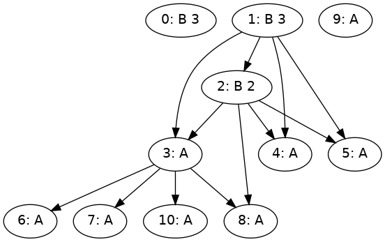
import Prelude (String)We’ll give our problem two kinds of tasks (A and B) and two kinds of resources (RA and RB).
data Task
 = A
 | B Time -- ^ A task of kind B has a known fixed runtime.
 deriving (Eq, Ord, Show)

data Resource = RA | RB deriving (Eq, Ord, Show)
Let’s declare that a task of kind A (resp. RB) can run on only on a resource of kind RA (resp. RB).
compatibility :: (Task, Resource) -> Bool
compatibility (A, RA) = True
compatibility ((B _), RB) = True
compatibility _ = False
In this particular case, task processing time for A is always one, and task processing time for B is a function of the task itself.
processingTime :: (Task, Resource) -> Time
processingTime (A, RA) = 1
processingTime ((B x), RB) = x
processingTime _ = (panic "runtime query on invalid placement")
We’ll identify tasks and resources via unique identifiers.
type TaskID = Int
type ResourceID = Int
For the sake of running GLPK, here’s an arbitrary problem instance:
exampleTasks :: Map TaskID Task
exampleTasks = M.fromList $
  [(0, B 3), (1, B 3), (2, B 2)]
  <> fmap (,A) [3 .. 10]

exampleResources :: Map ResourceID Resource
exampleResources = M.fromList [(0, RA), (1, RA), (2, RB)]

examplePrecedences :: Map TaskID [TaskID]
examplePrecedences = M.fromList
  [ (2, [4, 3, 8, 5])
  , (1, [4, 5, 2, 3])
  , (3, [7, 6, 8, 10])
  ]
Compatibility and runtime lookups can be implemented like so.
compatible :: TaskID -> ResourceID -> Bool
compatible tid rid =
  (M.lookup tid exampleTasks, M.lookup rid exampleResources) & \case
    (Just t, Just r) -> compatibility (t, r)
    _ -> panic "unknown Task or Resource ID"

runtime :: TaskID -> ResourceID -> Time
runtime tid rid =
  (M.lookup tid exampleTasks, M.lookup rid exampleResources) & \case
    (Just t, Just r) -> processingTime (t, r)
    _ -> panic "unknown Task or Resource ID"
The corresponding ILP program can then be constructed via formulation.
testProgramBuilder ::
  Set TaskID ->
  Set ResourceID ->
  Map TaskID [TaskID] ->
  LP String Int
testProgramBuilder _J _R _P =
  formulation _J _R _P compatible runtime 20
Solving this program via GLPK results in the following log and schedule:
Solving and plotting code
prettyAssignment :: (Show job, Show resource) => (job, resource, Double) -> Text
prettyAssignment (j, r, t) =
  "t=" <> show t <> " scheduling task " <> show j <> " on " <> show r

prettySolved ::
  (Show job, Show resource) =>
  [job] ->
  [resource] ->
  Map String Double ->
  [(job, resource, Double)]
prettySolved jobs resources solved = mconcat listAssignments
  where
    listAssignments = cartesian jobs resources
      <&> \(j, r) -> M.lookup (allocated (j, r)) solved & \case
        Nothing -> []
        Just 1 ->
          let t = M.lookup (startTime j) solved & \case
                Nothing -> panic "s_j should exist for all j!"
                Just x -> x
           in [(j, r, t)]
        Just 0 -> []
        Just {} -> panic "x_j should be binary for all j!"

problemToPng :: Map TaskID a -> Map TaskID [TaskID] -> FilePath -> IO ()
problemToPng exTasks exPrecedences fn =
  void $
    runGraphviz
      ( graphToDot
          quickParams
          (toGraph (toList (M.keys exTasks)) (exPrecedences))
      )
      Png
      fn

example :: IO ()
example = do
  problemToPng exampleTasks examplePrecedences "exampleProblem.png"
  let testProblem' =
        testProgramBuilder
          (S.fromList $ M.keys exampleTasks)
          (S.fromList $ M.keys exampleResources)
          examplePrecedences
  writeLP "example.ilp" testProblem'
  putText "solving LP!"
  lowerbound <- glpSolveVars
    (simplexDefaults {msgLev = MsgOff})
    (testProblem' {varTypes = varTypes testProblem' <&> const ContVar})
    >>= \case
      (Success, Just (x, _)) -> return x
      _ -> panic "LP relaxation, solving failed"
  glpSolveVars (mipDefaults {tmLim = 500}) testProblem' >>= \case
    (returnCode, Just (_, solved)) -> do
      print returnCode
      putText $
        "Solved program with "
          <> show (length solved)
          <> " variables."
      let assignments :: [(TaskID, ResourceID, Double)]
          assignments =
            sortBy
              (\(_, _, t) (_, _, t') -> compare t t')
              ( prettySolved (M.keys exampleTasks) (M.keys exampleResources) solved
              )
          formatted :: Text
          formatted =
            mconcat . mconcat $
              (: ["\n"])
                <$> (prettyAssignment <$> assignments)
      void $ renderableToFile def "schedule.png"
        $ fillBackground def
        $ layoutToRenderable
        $ gantt assignments examplePrecedences lowerbound
      print assignments
      writeFile "output.txt" $ toS formatted
    _ -> panic "failure"

instance {-# OVERLAPPABLE #-} Show a => Labellable a where
  toLabelValue x = StrLabel (show x)

toGraph :: [TaskID] -> Map TaskID [TaskID] -> Gr Text Text
toGraph nodes' edges' =
  mkGraph
    ( nodes' <&> \tid ->
        ( tid,
          show tid <> ": " <> (show . fromJust $ M.lookup tid exampleTasks)
        )
    )
    (expandMap edges' <&> \(i, j) -> (i, j, ""))

intToDouble :: Int -> Double
intToDouble = fromInteger . Protolude.toInteger

gantt ::
  [(TaskID, ResourceID, Double)] ->
  Map TaskID [TaskID] ->
  Double ->
  Layout Double Double
gantt assignments precedences lowerbound = layout
  where
    dp :: Double
    dp = 0.35
    taskMap :: Map TaskID (ResourceID, Double)
    taskMap = M.fromList (assignments <&> \(t, r, d) -> (t, (r, d)))
    resourceValue :: ResourceID -> Double
    resourceValue i = fromInteger $ Protolude.toInteger i
    precedenceVectors :: [((Double, Double), (Double, Double))]
    precedenceVectors = mconcat $
      M.toList precedences <&> \(tid, tids) ->
        pVector tid <$> tids
    pVector :: TaskID -> TaskID -> ((Double, Double), (Double, Double))
    pVector i i' = ((ti + rt - dp, ri), (ti' - ti - rt + dp * 2, ri' - ri))
      where
        rt = (intToDouble $ runtime i rid)
        (rid@(resourceValue -> ri), ti) = fromJust $ M.lookup i taskMap
        (resourceValue -> ri', ti') = fromJust $ M.lookup i' taskMap
    bound =
      plot_lines_values .~ [[(lowerbound, -1 :: Double), (lowerbound, 4)]]
        $ plot_lines_style .~ dashedLine 1.5 [2, 2] (withOpacity C.red 1)
        $ def
    vals :: [((Double, Double), (Double, Double))]
    vals = assignments <&> \(t, r, s) ->
      let x = fromIntegral $ fromJust (elemIndex r (M.keys exampleResources))
          p = fromIntegral (runtime t r)
       in ((s + dp, x), (p -2 * dp, 0))
    annot =
      plot_annotation_values
        .~ [ (d + 0.2, - 0.05 + fromIntegral (fromJust (elemIndex r (M.keys exampleResources))), show t)
             | (t, r, d) <- assignments
           ]
        $ def
    prefVectors =
      plot_vectors_values .~ precedenceVectors
        $ plot_vectors_scale .~ 0
        $ plot_vectors_style . vector_line_style
          .~ dashedLine 1.5 [2, 2] (withOpacity black 1)
        $ plot_vectors_style . vector_head_style . point_color .~ withOpacity black 1
        $ def
    taskVectors =
      plot_vectors_values .~ vals
        $ plot_vectors_scale .~ 0
        $ plot_vectors_style . vector_line_style . line_width .~ 40
        $ plot_vectors_style . vector_line_style . line_color
          .~ withOpacity black 0.1
        $ plot_vectors_style . vector_head_style . point_radius .~ 0
        $ def
    layout =
      layout_title .~ "solution"
        $ layout_x_axis . laxis_override
          .~ ( const $
                 makeAxis
                   ( fmap
                       ( (\x -> if x >= 0 then show x else "")
                           . (round :: Double -> Integer)
                       )
                   )
                   ( [0 .. 10],
                     [],
                     [0 .. 10]
                   )
             )
        $ layout_y_axis . laxis_override
          .~ ( const $
                 makeAxis
                   ( fmap
                       \x -> M.lookup x (M.mapKeys intToDouble exampleResources)
                         & \case
                           Nothing -> ""
                           Just l -> show ((round x) :: Integer) <> ":" <> show l
                   )
                   ( [-0.5] <> (M.keys exampleResources <&> \ i -> fromInteger $ Protolude.toInteger i) <> [2.5] :: [Double],
                     vals <&> \((x, _), _) -> x,
                     [0, 1, 2] :: [Double]
                   )
             )
        $ layout_left_axis_visibility . axis_show_ticks .~ False
        $ layout_plots
          .~ [ plotVectorField taskVectors,
               toPlot annot,
               toPlot bound,
               plotVectorField prefVectors
             ]
        $ def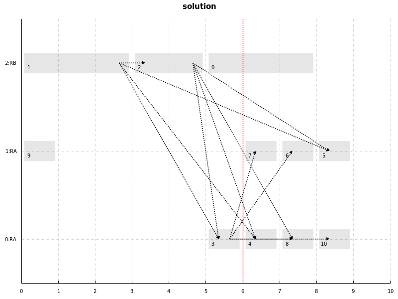
We won the ILP lottery: GLPK terminated (in a few seconds). Because this is the case, we know the solution obtained to be optimal. The red bar on the graph is the bound obtained by running the relaxed version of the problem, where all variables are made continuous. As explained, this is a lower bound of the solution that can always be computed efficiently.